18. The Aiyagari Model#
GPU
This lecture was built using a machine with JAX installed and access to a GPU.
To run this lecture on Google Colab, click on the “play” icon top right, select Colab, and set the runtime environment to include a GPU.
To run this lecture on your own machine, you need to install Google JAX.
18.1. Overview#
In this lecture, we describe the structure of a class of models that build on work by Truman Bewley [Bew77].
We begin by discussing an example of a Bewley model due to Rao Aiyagari [Aiy94].
The model features
Heterogeneous agents
A single exogenous vehicle for borrowing and lending
Limits on amounts individual agents may borrow
The Aiyagari model has been used to investigate many topics, including
precautionary savings and the effect of liquidity constraints [Aiy94]
risk sharing and asset pricing [HL96]
the shape of the wealth distribution [BBZ15]
18.1.1. References#
The primary reference for this lecture is [Aiy94].
A textbook treatment is available in chapter 18 of [LS18].
A less sophisticated version of this lecture (without JAX) can be found here.
18.1.2. Preliminaries#
We use the following imports
import time
import matplotlib.pyplot as plt
import numpy as np
import jax
import jax.numpy as jnp
from collections import namedtuple
Let’s check the GPU we are running
!nvidia-smi
/opt/conda/envs/quantecon/lib/python3.11/pty.py:89: RuntimeWarning: os.fork() was called. os.fork() is incompatible with multithreaded code, and JAX is multithreaded, so this will likely lead to a deadlock.
  pid, fd = os.forkpty()
Thu Apr 11 21:56:14 2024
+-----------------------------------------------------------------------------+
| NVIDIA-SMI 470.182.03   Driver Version: 470.182.03   CUDA Version: 12.3     |
|-------------------------------+----------------------+----------------------+
| GPU  Name        Persistence-M| Bus-Id        Disp.A | Volatile Uncorr. ECC |
| Fan  Temp  Perf  Pwr:Usage/Cap|         Memory-Usage | GPU-Util  Compute M. |
|                               |                      |               MIG M. |
|===============================+======================+======================|
|   0  Tesla V100-SXM2...  Off  | 00000000:00:1E.0 Off |                    0 |
| N/A   41C    P0    42W / 300W |      0MiB / 16160MiB |      2%      Default |
|                               |                      |                  N/A |
+-------------------------------+----------------------+----------------------+

+-----------------------------------------------------------------------------+
| Processes:                                                                  |
|  GPU   GI   CI        PID   Type   Process name                  GPU Memory |
|        ID   ID                                                   Usage      |
|=============================================================================|
|  No running processes found                                                 |
+-----------------------------------------------------------------------------+
We will use 64 bit floats with JAX in order to increase the precision.
jax.config.update("jax_enable_x64", True)
We will use the following function to compute stationary distributions of stochastic matrices. (For a reference to the algorithm, see p. 88 of Economic Dynamics.)
# Compute the stationary distribution of P by matrix inversion.

@jax.jit
def compute_stationary(P):
    n = P.shape[0]
    I = jnp.identity(n)
    O = jnp.ones((n, n))
    A = I - jnp.transpose(P) + O
    return jnp.linalg.solve(A, jnp.ones(n))
18.2. Firms#
Firms produce output by hiring capital and labor.
Firms act competitively and face constant returns to scale.
Since returns to scale are constant the number of firms does not matter.
Hence we can consider a single (but nonetheless competitive) representative firm.
The firm’s output is
where
\( A \) and \( \alpha \) are parameters with \( A > 0 \) and \( \alpha \in (0, 1) \)
\( K_t \) is aggregate capital
\( N \) is total labor supply (which is constant in this simple version of the model)
The firm’s problem is
The parameter \( \delta \) is the depreciation rate.
These parameters are stored in the following namedtuple.
Firm = namedtuple('Firm', ('A', 'N', 'α', 'β', 'δ'))

def create_firm(A=1.0,
                N=1.0,
                α=0.33,
                β=0.96,
                δ=0.05):

    return Firm(A=A, N=N, α=α, β=β, δ=δ)
From the first-order condition with respect to capital,
the firm’s inverse demand for capital is
def r_given_k(K, firm):
    """
    Inverse demand curve for capital.  The interest rate associated with a
    given demand for capital K.
    """
    A, N, α, β, δ = firm
    return A * α * (N / K)**(1 - α) - δ
Using (18.1) and the firm’s first-order condition for labor,
we can pin down the equilibrium wage rate as a function of \( r \) as
def r_to_w(r, f):
    """
    Equilibrium wages associated with a given interest rate r.
    """
    A, N, α, β, δ = f
    return A * (1 - α) * (A * α / (r + δ))**(α / (1 - α))
18.3. Households#
Infinitely lived households / consumers face idiosyncratic income shocks.
A unit interval of ex-ante identical households face a common borrowing constraint.
The savings problem faced by a typical household is
subject to
where
\( c_t \) is current consumption
\( a_t \) is assets
\( z_t \) is an exogenous component of labor income capturing stochastic unemployment risk, etc.
\( w \) is a wage rate
\( r \) is a net interest rate
\( B \) is the maximum amount that the agent is allowed to borrow
The exogenous process \( \{z_t\} \) follows a finite state Markov chain with given stochastic matrix \( P \).
In this simple version of the model, households supply labor inelastically because they do not value leisure.
Below we provide code to solve the household problem, taking \(r\) and \(w\) as fixed.
For now we assume that \(u(c) = \log(c)\).
(CRRA utility is treated in the exercises.)
18.3.1. Primitives and Operators#
This namedtuple stores the parameters that define a household asset accumulation problem and the grids used to solve it.
Household = namedtuple('Household', ('r', 'w', 'β', 'a_size', 'z_size', \
                                     'a_grid', 'z_grid', 'Π'))

def create_household(r=0.01,                      # Interest rate
                     w=1.0,                       # Wages
                     β=0.96,                      # Discount factor
                     Π=[[0.9, 0.1], [0.1, 0.9]],  # Markov chain
                     z_grid=[0.1, 1.0],           # Exogenous states
                     a_min=1e-10, a_max=20,       # Asset grid
                     a_size=200):

    a_grid = jnp.linspace(a_min, a_max, a_size)
    z_grid, Π = map(jnp.array, (z_grid, Π))
    Π = jax.device_put(Π)
    z_grid = jax.device_put(z_grid)
    z_size = len(z_grid)
    a_grid, z_grid, Π = jax.device_put((a_grid, z_grid, Π))

    return Household(r=r, w=w, β=β, a_size=a_size, z_size=z_size, \
                     a_grid=a_grid, z_grid=z_grid, Π=Π)
def u(c):
    return jnp.log(c)
This is the vectorized version of the right-hand side of the Bellman equation (before maximization), which is a 3D array representing
for all \((a, z, a')\).
def B(v, constants, sizes, arrays):
    # Unpack
    r, w, β = constants
    a_size, z_size = sizes
    a_grid, z_grid, Π = arrays

    # Compute current consumption as array c[i, j, ip]
    a  = jnp.reshape(a_grid, (a_size, 1, 1))    # a[i]   ->  a[i, j, ip]
    z  = jnp.reshape(z_grid, (1, z_size, 1))    # z[j]   ->  z[i, j, ip]
    ap = jnp.reshape(a_grid, (1, 1, a_size))    # ap[ip] -> ap[i, j, ip]
    c = w*z + (1 + r)*a - ap

    # Calculate continuation rewards at all combinations of (a, z, ap)
    v = jnp.reshape(v, (1, 1, a_size, z_size))  # v[ip, jp] -> v[i, j, ip, jp]
    Π = jnp.reshape(Π, (1, z_size, 1, z_size))  # Π[j, jp]  -> Π[i, j, ip, jp]
    EV = jnp.sum(v * Π, axis=3)                 # sum over last index jp

    # Compute the right-hand side of the Bellman equation
    return jnp.where(c > 0, u(c) + β * EV, -jnp.inf)

B = jax.jit(B, static_argnums=(2,))
The next function computes greedy policies.
# Computes a v-greedy policy, returned as a set of indices
def get_greedy(v, constants, sizes, arrays):
    return jnp.argmax(B(v, constants, sizes, arrays), axis=2)

get_greedy = jax.jit(get_greedy, static_argnums=(2,))
We need to know rewards at a given policy for policy iteration.
The following functions computes the array \(r_{\sigma}\) which gives current rewards given policy \(\sigma\).
That is,
def compute_r_σ(σ, constants, sizes, arrays):
    # Unpack
    r, w, β = constants
    a_size, z_size = sizes
    a_grid, z_grid, Π = arrays

    # Compute r_σ[i, j]
    a = jnp.reshape(a_grid, (a_size, 1))
    z = jnp.reshape(z_grid, (1, z_size))
    ap = a_grid[σ]
    c = (1 + r)*a + w*z - ap
    r_σ = u(c)

    return r_σ

compute_r_σ = jax.jit(compute_r_σ, static_argnums=(2,))
The value \(v_{\sigma}\) of a policy \(\sigma\) is defined as
Here we set up the linear map \(v \rightarrow R_{\sigma} v\), where \(R_{\sigma} := I - \beta P_{\sigma}\).
In the consumption problem, this map can be expressed as
Defining the map as above works in a more intuitive multi-index setting
(e.g. working with \(v[i, j]\) rather than flattening \(v\) to a one-dimensional array)
and avoids instantiating the large matrix \(P_{\sigma}\).
def R_σ(v, σ, constants, sizes, arrays):
    # Unpack
    r, w, β = constants
    a_size, z_size = sizes
    a_grid, z_grid, Π = arrays

    # Set up the array v[σ[i, j], jp]
    zp_idx = jnp.arange(z_size)
    zp_idx = jnp.reshape(zp_idx, (1, 1, z_size))
    σ = jnp.reshape(σ, (a_size, z_size, 1))
    V = v[σ, zp_idx]

    # Expand Π[j, jp] to Π[i, j, jp]
    Π = jnp.reshape(Π, (1, z_size, z_size))

    # Compute and return v[i, j] - β Σ_jp v[σ[i, j], jp] * Π[j, jp]
    return v - β * jnp.sum(V * Π, axis=2)

R_σ = jax.jit(R_σ, static_argnums=(3,))
The next function computes the lifetime value of a given policy.
# Get the value v_σ of policy σ by inverting the linear map R_σ

def get_value(σ, constants, sizes, arrays):

    r_σ = compute_r_σ(σ, constants, sizes, arrays)
    # Reduce R_σ to a function in v
    partial_R_σ = lambda v: R_σ(v, σ, constants, sizes, arrays)
    # Compute inverse v_σ = (I - β P_σ)^{-1} r_σ
    return jax.scipy.sparse.linalg.bicgstab(partial_R_σ, r_σ)[0]

get_value = jax.jit(get_value, static_argnums=(2,))
18.4. Solvers#
We will solve the household problem using Howard policy iteration.
def policy_iteration(household, tol=1e-4, max_iter=10_000, verbose=False):
    """Howard policy iteration routine."""

    γ, w, β, a_size, z_size, a_grid, z_grid, Π = household

    constants = γ, w, β
    sizes = a_size, z_size
    arrays = a_grid, z_grid, Π

    σ = jnp.zeros(sizes, dtype=int)
    v_σ = get_value(σ, constants, sizes, arrays)
    i = 0
    error = tol + 1
    while error > tol and i < max_iter:
        σ_new = get_greedy(v_σ, constants, sizes, arrays)
        v_σ_new = get_value(σ_new, constants, sizes, arrays)
        error = jnp.max(jnp.abs(v_σ_new - v_σ))
        σ = σ_new
        v_σ = v_σ_new
        i = i + 1
        if verbose:
            print(f"Concluded loop {i} with error {error}.")
    return σ
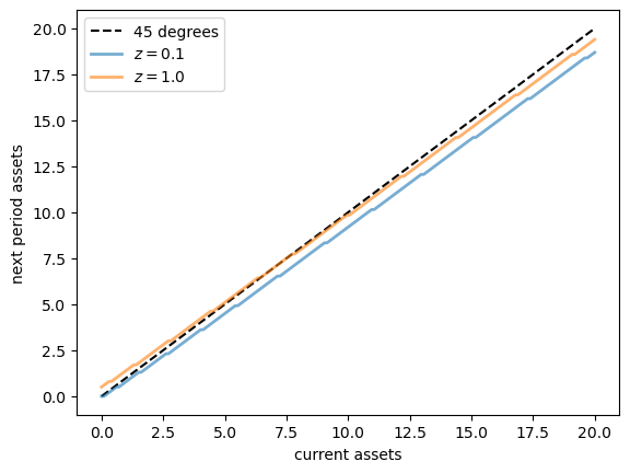
As a first example of what we can do, let’s compute and plot an optimal accumulation policy at fixed prices.
# Create an instance of Housbehold
household = create_household()
%%time

σ_star = policy_iteration(household, verbose=True)


# The next plot shows asset accumulation policies at different values of the exogenous state.
Concluded loop 1 with error 11.366831579022996.
Concluded loop 2 with error 9.574522771860245.
Concluded loop 3 with error 3.9654760004604777.
Concluded loop 4 with error 1.1207075306313232.
Concluded loop 5 with error 0.2524013153055833.
Concluded loop 6 with error 0.12172293662906064.
Concluded loop 7 with error 0.043395682867316765.
Concluded loop 8 with error 0.012132319676439351.
Concluded loop 9 with error 0.005822155404443308.
Concluded loop 10 with error 0.002863165320343697.
Concluded loop 11 with error 0.0016657175376657563.
Concluded loop 12 with error 0.0004143776102245589.
Concluded loop 13 with error 0.0.
CPU times: user 617 ms, sys: 52.4 ms, total: 669 ms
Wall time: 821 ms
γ, w, β, a_size, z_size, a_grid, z_grid, Π = household

fig, ax = plt.subplots()
ax.plot(a_grid, a_grid, 'k--', label="45 degrees")
for j, z in enumerate(z_grid):
    lb = f'$z = {z:.2}$'
    policy_vals = a_grid[σ_star[:, j]]
    ax.plot(a_grid, policy_vals, lw=2, alpha=0.6, label=lb)
    ax.set_xlabel('current assets')
    ax.set_ylabel('next period assets')
ax.legend(loc='upper left')
plt.show()
18.4.1. Capital Supply#
To start thinking about equilibrium, we need to know how much capital households supply at a given interest rate \(r\).
This quantity can be calculated by taking the stationary distribution of assets under the optimal policy and computing the mean.
The next function implements this calculation for a given policy \(\sigma\).
First we compute the stationary distribution of \(P_{\sigma}\), which is for the bivariate Markov chain of the state \((a_t, z_t)\). Then we sum out \(z_t\) to get the marginal distribution for \(a_t\).
def compute_asset_stationary(σ, constants, sizes, arrays):

    # Unpack
    r, w, β = constants
    a_size, z_size = sizes
    a_grid, z_grid, Π = arrays

    # Construct P_σ as an array of the form P_σ[i, j, ip, jp]
    ap_idx = jnp.arange(a_size)
    ap_idx = jnp.reshape(ap_idx, (1, 1, a_size, 1))
    σ = jnp.reshape(σ, (a_size, z_size, 1, 1))
    A = jnp.where(σ == ap_idx, 1, 0)
    Π = jnp.reshape(Π, (1, z_size, 1, z_size))
    P_σ = A * Π

    # Reshape P_σ into a matrix
    n = a_size * z_size
    P_σ = jnp.reshape(P_σ, (n, n))

    # Get stationary distribution and reshape onto [i, j] grid
    ψ = compute_stationary(P_σ)
    ψ = jnp.reshape(ψ, (a_size, z_size))

    # Sum along the rows to get the marginal distribution of assets
    ψ_a = jnp.sum(ψ, axis=1)
    return ψ_a

compute_asset_stationary = jax.jit(compute_asset_stationary,
                                   static_argnums=(2,))
Let’s give this a test run.
γ, w, β, a_size, z_size, a_grid, z_grid, Π = household
constants = γ, w, β
sizes = a_size, z_size
arrays = a_grid, z_grid, Π
ψ = compute_asset_stationary(σ_star, constants, sizes, arrays)
The distribution should sum to one:
ψ.sum()
Array(1., dtype=float64)
Now we are ready to compute capital supply by households given wages and interest rates.
def capital_supply(household):
    """
    Map household decisions to the induced level of capital stock.
    """

    # Unpack
    γ, w, β, a_size, z_size, a_grid, z_grid, Π = household

    constants = γ, w, β
    sizes = a_size, z_size
    arrays = a_grid, z_grid, Π

    # Compute the optimal policy
    σ_star = policy_iteration(household)
    # Compute the stationary distribution
    ψ_a = compute_asset_stationary(σ_star, constants, sizes, arrays)

    # Return K
    return float(jnp.sum(ψ_a * a_grid))
18.5. Equilibrium#
We construct a stationary rational expectations equilibrium (SREE).
In such an equilibrium
prices induce behavior that generates aggregate quantities consistent with the prices
aggregate quantities and prices are constant over time
In more detail, an SREE lists a set of prices, savings and production policies such that
households want to choose the specified savings policies taking the prices as given
firms maximize profits taking the same prices as given
the resulting aggregate quantities are consistent with the prices; in particular, the demand for capital equals the supply
aggregate quantities (defined as cross-sectional averages) are constant
In practice, once parameter values are set, we can check for an SREE by the following steps
pick a proposed quantity \( K \) for aggregate capital
determine corresponding prices, with interest rate \( r \) determined by (18.1) and a wage rate \( w(r) \) as given in (18.2).
determine the common optimal savings policy of the households given these prices
compute aggregate capital as the mean of steady state capital given this savings policy
If this final quantity agrees with \( K \) then we have a SREE. Otherwise we adjust \(K\).
These steps describe a fixed point problem which we solve below.
18.5.1. Visual inspection#
Let’s inspect visually as a first pass.
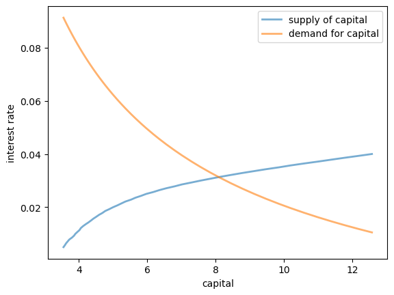
The following code draws aggregate supply and demand curves for capital.
The intersection gives equilibrium interest rates and capital.
# Create default instances
household = create_household()
firm = create_firm()

# Create a grid of r values at which to compute demand and supply of capital
num_points = 50
r_vals = np.linspace(0.005, 0.04, num_points)
%%time

# Compute supply of capital
k_vals = np.empty(num_points)
for i, r in enumerate(r_vals):
    # _replace create a new nametuple with the updated parameters
    household = household._replace(r=r, w=r_to_w(r, firm))
    k_vals[i] = capital_supply(household)
CPU times: user 3.75 s, sys: 899 ms, total: 4.65 s
Wall time: 2.69 s
# Plot against demand for capital by firms

fig, ax = plt.subplots()
ax.plot(k_vals, r_vals, lw=2, alpha=0.6, label='supply of capital')
ax.plot(k_vals, r_given_k(k_vals, firm), lw=2, alpha=0.6, label='demand for capital')
ax.set_xlabel('capital')
ax.set_ylabel('interest rate')
ax.legend(loc='upper right')

plt.show()
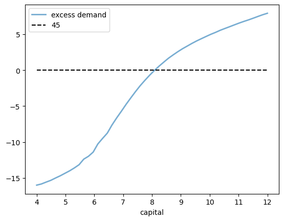
Here’s a plot of the excess demand function.
The equilibrium is the zero (root) of this function.
def excess_demand(K, firm, household):
    r = r_given_k(K, firm)
    w = r_to_w(r, firm)
    household = household._replace(r=r, w=w)
    return K - capital_supply(household)
%%time

num_points = 50
k_vals = np.linspace(4, 12, num_points)
out = [excess_demand(k, firm, household) for k in k_vals]
CPU times: user 3.32 s, sys: 955 ms, total: 4.27 s
Wall time: 2.28 s
fig, ax = plt.subplots()
ax.plot(k_vals, out, lw=2, alpha=0.6, label='excess demand')
ax.plot(k_vals, np.zeros_like(k_vals), 'k--', label="45")
ax.set_xlabel('capital')
ax.legend()
plt.show()
18.5.2. Computing the equilibrium#
Now let’s compute the equilibrium
To do so, we use the bisection method, which is implemented in the next function.
def bisect(f, a, b, *args, tol=10e-2):
    """
    Implements the bisection root finding algorithm, assuming that f is a
    real-valued function on [a, b] satisfying f(a) < 0 < f(b).
    """
    lower, upper = a, b
    count = 0
    while upper - lower > tol and count < 10000:
        middle = 0.5 * (upper + lower)
        if f(middle, *args) > 0:   # root is between lower and middle
            lower, upper = lower, middle
        else:                      # root is between middle and upper
            lower, upper = middle, upper
        count += 1
    if count == 10000:
        print("Root might not be accurate")
    return 0.5 * (upper + lower), count
Now we call the bisection function on excess demand.
def compute_equilibrium(firm, household):
    print("\nComputing equilibrium capital stock")
    start = time.time()
    solution, count = bisect(excess_demand, 6.0, 10.0, firm, household)
    elapsed = time.time() - start
    print(f"Computed equilibrium in {count} iterations and {elapsed} seconds")
    return solution
%%time

household = create_household()
firm = create_firm()
compute_equilibrium(firm, household)
Computing equilibrium capital stock
Computed equilibrium in 6 iterations and 0.28626155853271484 seconds
CPU times: user 406 ms, sys: 133 ms, total: 539 ms
Wall time: 288 ms
8.09375
Notice how quickly we can compute the equilibrium capital stock using a simple method such as bisection.
18.6. Exercises#
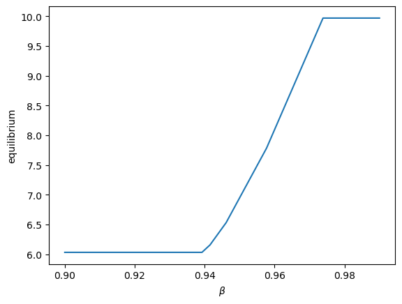
Exercise 18.1
Using the default household and firm model, produce a graph showing the behaviour of equilibrium capital stock with the increase in \(\beta\).
Solution to Exercise 18.1
β_vals = np.linspace(0.9, 0.99, 40)
eq_vals = np.empty_like(β_vals)

for i, β in enumerate(β_vals):
    household = create_household(β=β)
    firm = create_firm(β=β)
    eq_vals[i] = compute_equilibrium(firm, household)
Computing equilibrium capital stock
Computed equilibrium in 6 iterations and 0.6101107597351074 seconds

Computing equilibrium capital stock
Computed equilibrium in 6 iterations and 0.1564176082611084 seconds

Computing equilibrium capital stock
Computed equilibrium in 6 iterations and 0.162703275680542 seconds

Computing equilibrium capital stock
Computed equilibrium in 6 iterations and 0.16426849365234375 seconds

Computing equilibrium capital stock
Computed equilibrium in 6 iterations and 0.17319059371948242 seconds

Computing equilibrium capital stock
Computed equilibrium in 6 iterations and 0.16875004768371582 seconds

Computing equilibrium capital stock
Computed equilibrium in 6 iterations and 0.1761479377746582 seconds

Computing equilibrium capital stock
Computed equilibrium in 6 iterations and 0.1830596923828125 seconds

Computing equilibrium capital stock
Computed equilibrium in 6 iterations and 0.17809367179870605 seconds

Computing equilibrium capital stock
Computed equilibrium in 6 iterations and 0.18584346771240234 seconds

Computing equilibrium capital stock
Computed equilibrium in 6 iterations and 0.20784449577331543 seconds

Computing equilibrium capital stock
Computed equilibrium in 6 iterations and 0.1989436149597168 seconds
Computing equilibrium capital stock
Computed equilibrium in 6 iterations and 0.2059495449066162 seconds

Computing equilibrium capital stock
Computed equilibrium in 6 iterations and 0.2235887050628662 seconds

Computing equilibrium capital stock
Computed equilibrium in 6 iterations and 0.21914124488830566 seconds

Computing equilibrium capital stock
Computed equilibrium in 6 iterations and 0.23400402069091797 seconds

Computing equilibrium capital stock
Computed equilibrium in 6 iterations and 0.22857093811035156 seconds

Computing equilibrium capital stock
Computed equilibrium in 6 iterations and 0.23694181442260742 seconds

Computing equilibrium capital stock
Computed equilibrium in 6 iterations and 0.24532270431518555 seconds

Computing equilibrium capital stock
Computed equilibrium in 6 iterations and 0.25931620597839355 seconds

Computing equilibrium capital stock
Computed equilibrium in 6 iterations and 0.24804973602294922 seconds

Computing equilibrium capital stock
Computed equilibrium in 6 iterations and 0.26594114303588867 seconds

Computing equilibrium capital stock
Computed equilibrium in 6 iterations and 0.25882506370544434 seconds

Computing equilibrium capital stock
Computed equilibrium in 6 iterations and 0.2736814022064209 seconds

Computing equilibrium capital stock
Computed equilibrium in 6 iterations and 0.28816819190979004 seconds

Computing equilibrium capital stock
Computed equilibrium in 6 iterations and 0.30350732803344727 seconds

Computing equilibrium capital stock
Computed equilibrium in 6 iterations and 0.2843303680419922 seconds

Computing equilibrium capital stock
Computed equilibrium in 6 iterations and 37.14894390106201 seconds

Computing equilibrium capital stock
Computed equilibrium in 6 iterations and 0.31118106842041016 seconds

Computing equilibrium capital stock
Computed equilibrium in 6 iterations and 0.2965826988220215 seconds

Computing equilibrium capital stock
Computed equilibrium in 6 iterations and 0.2880594730377197 seconds

Computing equilibrium capital stock
Computed equilibrium in 6 iterations and 0.30828261375427246 seconds

Computing equilibrium capital stock
Computed equilibrium in 6 iterations and 0.3152189254760742 seconds

Computing equilibrium capital stock
Computed equilibrium in 6 iterations and 0.33822131156921387 seconds

Computing equilibrium capital stock
Computed equilibrium in 6 iterations and 0.34753894805908203 seconds

Computing equilibrium capital stock
Computed equilibrium in 6 iterations and 0.3719043731689453 seconds

Computing equilibrium capital stock
Computed equilibrium in 6 iterations and 0.39298439025878906 seconds

Computing equilibrium capital stock
Computed equilibrium in 6 iterations and 0.4101893901824951 seconds

Computing equilibrium capital stock
Computed equilibrium in 6 iterations and 0.41483473777770996 seconds

Computing equilibrium capital stock
Computed equilibrium in 6 iterations and 0.42214536666870117 seconds
fig, ax = plt.subplots()
ax.plot(β_vals, eq_vals, ms=2)
ax.set_xlabel(r'$\beta$')
ax.set_ylabel('equilibrium')
plt.show()
Exercise 18.2
Switch to the CRRA utility function
and re-do the plot of demand for capital by firms against the supply of captial.
Also, recompute the equilibrium.
Use the default parameters for households and firms.
Set \(\gamma=2\).
Solution to Exercise 18.2
Let’s define the utility function
def u(c, γ=2):
    return c**(1 - γ) / (1 - γ)
We need to re-compile all the jitted functions in order notice the change in the utility function.
B = jax.jit(B, static_argnums=(2,))
get_greedy = jax.jit(get_greedy, static_argnums=(2,))
compute_r_σ = jax.jit(compute_r_σ, static_argnums=(2,))
R_σ = jax.jit(R_σ, static_argnums=(3,))
get_value = jax.jit(get_value, static_argnums=(2,))
compute_asset_stationary = jax.jit(compute_asset_stationary,
                                   static_argnums=(2,))
Now, let’s plot the the demand for capital by firms
# Create default instances
household = create_household()
firm = create_firm()

# Create a grid of r values at which to compute demand and supply of capital
num_points = 50
r_vals = np.linspace(0.005, 0.04, num_points)


# Compute supply of capital
k_vals = np.empty(num_points)
for i, r in enumerate(r_vals):
    household = household._replace(r=r, w=r_to_w(r, firm))
    k_vals[i] = capital_supply(household)
# Plot against demand for capital by firms

fig, ax = plt.subplots()
ax.plot(k_vals, r_vals, lw=2, alpha=0.6, label='supply of capital')
ax.plot(k_vals, r_given_k(k_vals, firm), lw=2, alpha=0.6, label='demand for capital')
ax.set_xlabel('capital')
ax.set_ylabel('interest rate')
ax.legend()

plt.show()
Compute the equilibrium
%%time

household = create_household()
firm = create_firm()
compute_equilibrium(firm, household)
Computing equilibrium capital stock
Computed equilibrium in 6 iterations and 0.6658434867858887 seconds
CPU times: user 890 ms, sys: 71.1 ms, total: 961 ms
Wall time: 667 ms
8.09375